 IntroductionData is the new oil of the 21st century [1]. Many data come from the web [2]. Acquiring these webdata and structuring them is called webscraping. In this blog, I will briefly discuss how to webscrape data. However, it does not stop there. Analyses beyond webscraping are often needed. Some additional steps are shown, such as capturing hidden characters, merging different data, summary stats and visualization. Luckily, Python can be used for the whole analysis pipeline. Healthcare data are used for the current purpose, but it should be mentioned that many data can be webscraped in a similar way, sometimes with a few adaptations in the code. Important note: webdata are dynamic. Please report me if code is not working, this may be due to changes in the downloaded web tables. The current blog has been updated in September 2018. A previous version was published in June 2017 at https://rrighart.github.io/ . The code is based on Python 2.7. Some minor changes may be needed for Python 3.4 and later versions. Healthcare rankings for different European countriesBeautiful Soup is a Python package that is used for webscraping [3]. In this blog we will scrape tables from webpages. First, we need to determine at which directory data will be saved. We are going to scrape data from Wikipedia [4]. The data indicate scores on different health indices, such as patient rights and information, accessibility (waiting time for treatment), outcomes, range and reach of services provided, prevention, and pharmaceuticals. The data are from the Euro Health Consumer index. 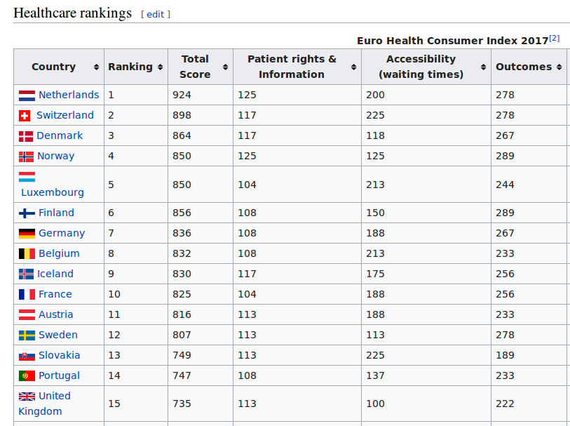 In the following code, we read the data and convert it to so-called bs4.BeautifulSoup data. Several data visualizations using Tableau can be found at my blog page [5]. We could display the data using print(HCE.prettify()). We will not do that here because it will produce a great amount of text (or soup). We first need to select the table that we'd like to scrape. As webpages often contain multiple tables, it would be good to read from the HTML the specific table names into a list [6]: The list lst has a length of 3: We will scrape the first table, and therefore use index 0 in lst to capture the first table name. The table will be read using Beautiful Soup's find function. A simple option is to type in the table name. You simply select the name in lst, which in this case is "wikitable sortable": Alternatively, there is a way to automate this step, by capturing the first data from the list, and then stripping off the unneeded characters. bs4.element.Tag It would be good to read in separately the header and row names, so we can easily make a DataFrame. [u'Country\n', u'Ranking\n', u'Total Score\n', u'Patient rights & Information\n', u'Accessibility (waiting times)\n', u'Outcomes\n', u'Range and reach of services provided\n', u'Prevention\n', u'Pharmaceuticals\n'] Now all element, - rows and headers -, are available to build the DataFrame, which we will call df1. 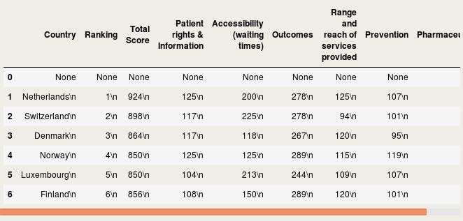 This table still needs a good amount of pre-processing, on which we will return later. Health expenditureOf course, other data sources can be scraped as well. So let us load data about health expenditure [7]. These are data per capita, which means that expenditure was corrected for the number of inhabitants in a country. Saving time, we will now put the script in one code block. This should lead to a DataFrame df2: <table class="wikitable sortable"> Let us inspect if the resulting DataFrame df2 looks fine:  Additional preprocessing stepsIf we look at the dataframes, we see that there are still some issues that prohibit numeric computations. There are undesired characters ('\n'), undesired decimal formats (comma should be removed), there are cells with non-numeric characters ('x' that should be NAN), and several columns should be numeric instead of object type. To resolve this, we will write a pre-processing function called preproc, which accepts as input any DataFrame (in our case df1 and df2). Please note that each web table may need its unique collection of pre-processing steps. Apparently, after the pre-processing there are some missing values (NANs): Now let us display where the NANs occur. In fact, when we check the original table, we can see that Cyprus has values "x", which were by our preproc function changed to NANs ( https://en.wikipedia.org/wiki/Healthcare_in_Europe ) 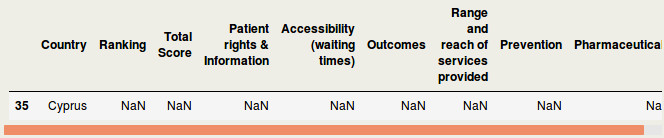 The following code will remove the NANs: At this point we inspect the data types: Honestly, the column names are a bit long. It would be good to use shorter names. Merging different dataIt should be clear from this example that webscraping can be important to quickly grasp data. Webscraping may be particularly useful when you need to automate data processing:
The health expenditure data give unexpected NANs. Something must be wrong here. We need to inspect this in more detail. Normally the set function should find a substantial overlap between countries in the two DataFrames. But it is empty. Strangely, there are several countries that are overlapping and there are no spelling errors. This suggests that the tables cannot merge because of a different reason. set() Let's inspect the two tables more closely. If we write the table to a csv file and check the raw text we may discover hidden symbols. If you now open the csv file in a spreadsheet software, you would discover that there are some hidden characters in the df1example.csv file. Using the repr function we can reveal the hidden characters [8]. '1 \xc2\xa0Netherlands\n2 \xc2\xa0\xc2\xa0Switzerland\n3 \xc2\xa0Denmark\n4 \xc2\xa0Norway\n5 \xc2\xa0Luxembourg\n6 \xc2\xa0Finland\n7 \xc2\xa0Germany\n8 \xc2\xa0Belgium\n9 \xc2\xa0Iceland\n10 \xc2\xa0France\n11 \xc2\xa0Austria\n12 \xc2\xa0Sweden\n13 \xc2\xa0Slovakia\n14 \xc2\xa0Portugal\n15 \xc2\xa0United Kingdom\n16 \xc2\xa0Slovenia\n17 \xc2\xa0Czechia\n18 \xc2\xa0Spain\n19 \xc2\xa0Estonia\n20 \xc2\xa0Serbia\n21 \xc2\xa0Italy\n22 \xc2\xa0Macedonia\n23 \xc2\xa0Malta\n24 \xc2\xa0Ireland\n25 \xc2\xa0Montenegro\n26 \xc2\xa0Croatia\n27 \xc2\xa0Albania\n28 \xc2\xa0Latvia\n29 \xc2\xa0Poland\n30 \xc2\xa0Hungary\n31 \xc2\xa0Lithuania\n32 \xc2\xa0Greece\n33 \xc2\xa0Bulgaria\n34 \xc2\xa0Romania\nName: Country, dtype: object' '1 Australia\n2 Austria\n3 Belgium\n4 Canada\n5 Chile\n6 Czech Republic\n7 Denmark\n8 Estonia\n9 Finland\n10 France\n11 Germany\n12 Greece\n13 Hungary\n14 Iceland\n15 Ireland\n16 Israel\n17 Italy\n18 Japan\n19 Korea\n20 Latvia\n21 Luxembourg\n22 Mexico\n23 Netherlands\n24 New Zealand\n25 Norway\n26 Poland\n27 Portugal\n28 Slovak Republic\n29 Slovenia\n30 Spain\n31 Sweden\n32 Switzerland\n33 Turkey\n34 United Kingdom\n35 United States\nName: Country, dtype: object' Luckily, all unwanted hidden characters are identical across the countries. That is, the characters are "\xc2\xa0" and "\n". Using the replace function we could remove this part. To inspect if it worked, we could re-use repr function and should see that the undesired characters are removed. Using the set function again we can see now that there are quite some countries that overlap: {'Austria', 'Belgium', 'Denmark', 'Estonia', 'Finland', 'France', 'Germany', 'Greece', 'Hungary', 'Iceland', 'Ireland', 'Italy', 'Latvia', 'Luxembourg', 'Netherlands', 'Norway', 'Poland', 'Portugal', 'Slovenia', 'Spain', 'Sweden', 'Switzerland', 'United Kingdom'} Now it is about time to merge the two tables. A few countries have NANs; in these cases for the expenditure data there were no values. We make a new DataFrame df3 from the merged data. After that we drop any rows where there are NANs. And we finally make a new DataFrame df3 from the merged data. After that we drop any rows where there are NANs. Data visualizationWe managed to bring the data together. The data are ready for analyses and visualization. We could visually inspect the relation between different variables using a scatterplot. The package adjustText takes care that the country labels do not overlap [9]. For the visualization, we will compute the average across years. We tune the axes and prepare the minimum and maximum values on the X- and Y-axis: Finally we can plot: 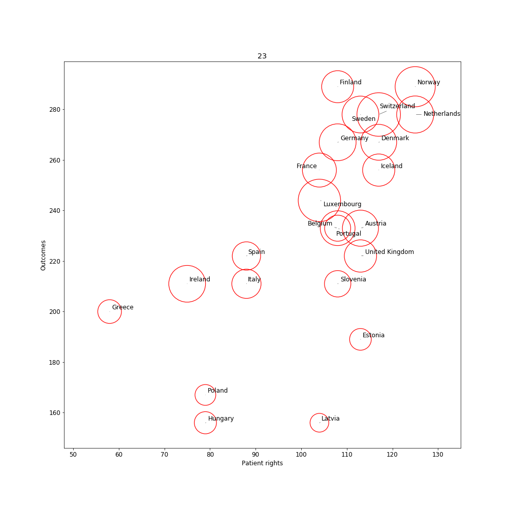 The visualization suggests a relation between patient rights and outcomes. Health expenditure is expressed by the diameter of the circles. The higher expenditure countries have better patient rights and outcomes (mostly in the right top corner). SummaryThe current blog showed how web tables can be scraped by using Python. A certain amount of pre-processing is necessary before these data can be visualized. Note that the world of web scraping is dynamic. The used websites and tables may be updated and therefore may require regular updates of Python code. Any questions or comments? Please feel free to contact me : Ruthger Righart E: [email protected] |W: https://www.rrighart.com References[1]. Data is the new oil. https://www.changethislimited.co.uk/2017/01/data-is-the-new-oil/
[2]. Data on internet. https://www.livescience.com/54094-how-big-is-the-internet.html [3]. Beautiful Soup. https://www.crummy.com/software/BeautifulSoup/bs4/ [4]. Healthcare Europe. https://en.wikipedia.org/wiki/Healthcare_in_Europe [5]. Visualizing European healthcare using Tableau. https://rrighart.github.io/HE-Tableau/ [6]. Scraping tables. https://stackoverflow.com/questions/17196018/extracting-table-contents-from-html-with-python-and-beautifulsoup [7]. Health expenditure. https://en.wikipedia.org/wiki/List_of_countries_by_total_health_expenditure_per_capita [8]. Hidden characters. https://stackoverflow.com/questions/31341351/how-can-i-identify-invisible-characters-in-python-strings [9]. Adjust text package. https://github.com/Phlya/adjustText/blob/master/examples/Examples.ipynb
0 Comments
|


|
Ruthger Righart
Ferney-Voltaire France Email: rrighart at googlemail dot com Tel.: 0033 (0)770071310 Immatriculation au Registre du Commerce et des Sociétés: 833 982 358 R.C.S. Bourg-en-Bresse. Greffe du Tribunal de Commerce, 32 Av Alsace Lorraine, 01011 Bourg-en-Bresse Cedex. |