PySpark in the context of sales data

Ruthger Righart
Data scientist

email: [email protected]
web: https://www.rrighart.com

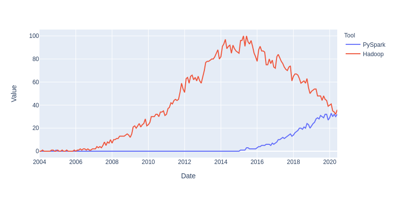
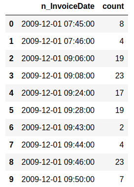
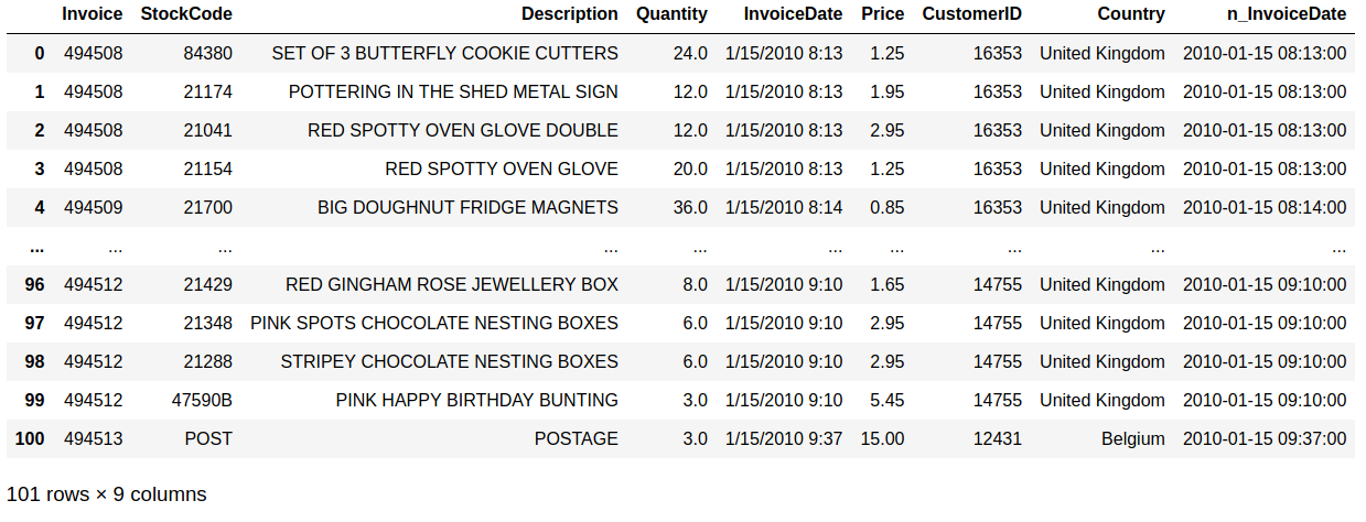
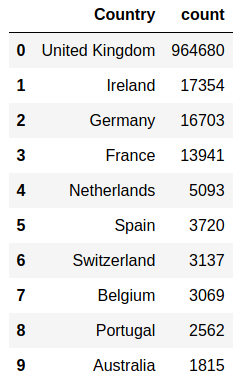
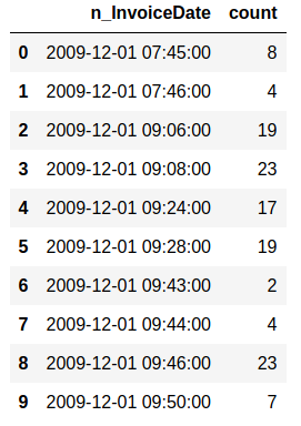
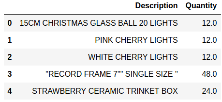
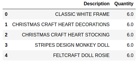
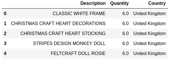
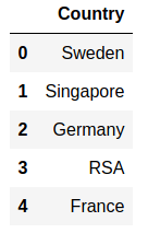
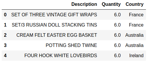
Sales and customer data provide important insight for companies. Analytics has today an important role in providing data about sales trends, customer profiles, warnings about (un)profitable products, sales volume forecasts and stock supply as well as personalizing customer relationships and giving product recommendations. All this information needs to be delivered in time, preferably in a (semi)automated fashion.

Photo by Stephen Dawson on Unsplash

These data can become large to the point that analytical tools and software have performance issues. For example, many businesses embrace spreadsheet software like Excel for understandable reasons, but it would breakdown with large data. Many data scientist work with Python/R, but modules like Pandas would become slow and run out of memory with large data as well.

Apache Spark enables large and big data analyses. It does this by using parallel processing using different threads and cores optimally. It can therefore improve performance on a cluster but also on a single machine [1]. It can do this for (i) unstructured data such as text or for (ii) structured data such as DataFrames arranged in columns. Spark does not require loading all data into memory before processing and it is faster than for example Hadoop.
Spark is a multi-language tool. Interfaces exist for Scala, Java, Python and R users, and it can be used in the cloud. These and other features make it a suitable platform for large scale data analyses. Google trends suggests that PySpark - Spark with a Python interface - enjoys increasing popularity.

Data source: Google Trends (https://www.google.com/trends).

The following blog shows a detailed short example using PySpark in the context of the Online retail sales data [2]. These are data that are arranged in column format, containing for example invoice number, invoice dates, quantity, price and product description. The chosen data serve as an example and the size would still work in Pandas for most single machine users, even though it would be slower.

The current blog does not provide a benchmark as done previously [1]. It rather gives hands-on analytical steps with code (i.e., concatenate data, removal of data records, renaming columns, replacing strings, casting data types, creation of new features, filtering data). It therefore allows a first glimpse into the world of PySpark.

START PYSPARK & IMPORT MODULES

The Jupyter notebook file PySpark-retaildata.ipynb  can be found at GitHub [3].
The notebook can be run in Google Colab. To install PySpark, type in the first cell !pip install pyspark .

An alternative is starting a Docker PySpark notebook [4].
After PySpark is installed and the Jupyter notebook is up and running, we first need to import the modules and create a Spark session:

Note that the Spark version used here is 2.4.5, which can be found by the command spark.version. At the writing of this text, 3.0.0. is being released.

LOADING AND DISPLAYING THE DATA

The Online retail data can be downloaded from the UCI machine learning repository [5]. The data sheets should be converted to online1.csv and online2.csv to facilitate loading from disk. The command pwd or os.getcwd() can be used to find the current directory from which PySpark will load the files. Below it can be seen that PySpark only takes a couple of seconds whereas Pandas would take a couple of minutes on the same machine.

Duration: 4.93 seconds

Duration: 1.75 seconds

Size of the DataFrames (or shapes in terms of Pandas) can be obtained with the following code:

To have all the data together in one DataFrame, df1 and df2 will be concatenated vertically.

The following displays the first 5 rows. The command .limit(5) will be used frequently throughout the text, which is comparable to the equivalent .head(5) in Pandas, to set the number of rows that is displayed.

This is the traditional Spark DataFrame output. By using the following setting we will get from now on a Pandas-like output.

A number of descriptive statistics can be obtained, like count, standard deviation, mean, minimum and maximum.

The table column count suggests that there are missing values in Description and Customer ID. The number of missing values is displayed by the following code:

Cancelled transactions start with a capital C in the column Invoice. These will be removed by the following.

The datashape function confirms that rows were removed.

Data shape (rows, columns): 1047877 x 8

CHANGING NAME AND DATA TYPE

The column name Customer ID contains an annoying white space that under certain circumstances can cause problems. So we should better rename that.

Further, the Country EIRE can be replaced by Ireland. The result can be verified by df.filter(df.Country == "Ireland").limit(5)

Information about the column type can be obtained. If you want some supplementary information, an alternative command is df.explain(df) .

StructType(List(StructField(Invoice,StringType,true),StructField(StockCode,StringType,true),StructField(Description,StringType,true),StructField(Quantity,IntegerType,true),StructField(InvoiceDate,StringType,true),StructField(Price,DoubleType,true),StructField(CustomerID,IntegerType,true),StructField(Country,StringType,true)))

Knowing the column types, we could now cast the column Quantity from integer to float.

The InvoiceDate shows up as a string. In order to exploit the time-related information, it would be best to convert it to date type. We will do this by creating a new column n_InvoiceDate.

Sorting the new dates, we can now display the number of records (rows) as a function of date and time.

It is also possible to display a range of dates. The following spots all sales at 15 Jan 2010 from 8 till 10 o'clock.

CONVERTING DATA

Time-serie analyses often require different units, like seconds, minutes, hours, days, weeks, months and years. For example, if we would like to display the sales per week, we could use the function weekofyear that translates the date to week.

Multiple columns can be used in a computation. The total Amount a customer spent can be computed by multiplication of the Price of a single product with its Quantity.

FILTERING DATA

How to select rows with specific products? We can use the command isin, which is very similar to the Pandas isin function:

If we want to search our data by key word, we would use the command like.

To find big buyers, probably organizational customers, select rows where Quantity is larger than 50000. Note that df.where(df.Quantity > 50000) would give a similar result.

Let us count the number of data records per country and sort the output, which shows that UK is clearly leading the list.

Sort can be used for InvoiceDate as well. This can show which hours customers purchase preferentially.

USING SQL IN PYSPARK

Luckily, Spark supports SQL - Structured Query Language - which traditionally has an important role in managing relational databases. Using for example SQL queries, a subset of the data can be exported to CRM and KPI sales software. This offers a lot of flexibility for data analyses. Let us experiment with some very useful SQL queries, such as select and filter. We first need to register the DataFrame as a temporary table in the SQLContext.

We first select a couple of columns, for example Description and Quantity. If you want to select all columns, simply use the star: spark.sql("select * from df").show(5)

Select the columns Description and Quantity and only those rows where Quantity has value = 6

Select the columns Description, Quantity, and Country where Quantity has value = 6 and country is United Kingdom.

SQL can also be used to show distinct (unique) values in a column. To limit space, only five are displayed here.

And we can count the number of distinct values, that is how many countries are in total in the data.

Using SQL we can also exclude certain values. For example, exclude all records with United Kingdom.

It would be possible to add a new column that categorizes UK (1) or not-UK (0). You could then use df.filter(df.Country == "United Kingdom").limit(5) and filter(df.Country == "France").limit(5) to check if the column is correctly coding UK versus not-UK.

Next, we could count UK versus not-UK using the new column Country_UK.

And compute mean Amount and summed Quantity.

FINAL THOUGHTS

That is it for now! In the current blog I have chosen to write out the code line by line. The code can of course be wrapped in several functions with the advantage that it can be used as a pre-processing script for different datasets, where you can set your own parameters. Further, smaller subsets of data can easily be exported and visualized in for ex. Plotly.

There are many other exciting features and developments in Spark:
1. Koalas is a Pandas API in Apache Spark, with similar capabilities but in a big data environment. This is particularly good news for people who already work in Pandas and need a quick translation to PySpark of their code.
2. Pandas UDF is a new feature that allows parallel processing on Pandas DataFrames.
3. There are excellent solutions using PySpark in the cloud. For example, AWS has big data platforms such as Elastic Map Reduce (EMR) that support PySpark.
4. Spark streaming allows real-time data analysis.
5. MLlib allows scalable machine learning in Spark.
6. GraphX enables graph computations.

If you have any questions or anything you think is missing in this tutorial, please feel free to share. Any suggestions for topics are welcome!

REFERENCES

[1] Chen, D., Laing Sain, S., Guo, K. (2012) Data mining for the online retail industry. A case study of RFM model-based customer segmentation using data mining. Journal of database marketing & customer strategy management, 19, 197-208.
[2] Wang, G., Xin, R., and Damji, J. (2018). Benchmarking Apache Spark on a single node machine. https://databricks.com/blog/2018/05/03/benchmarking-apache-spark-on-a-single-node-machine.html
[3] The Jupyter notebook file can be found at https://github.com/RRighart/Retail
[4] The Docker PySpark notebook can be found at https://github.com/jupyter/docker-stacks/tree/master/pyspark-notebook .
[5] The online retail data are at the UCI machine learning repository.